14 Measurement of Classical Gravitation Fields

Because of the principle of equivalence, one cannot ascribe a direct physical interpretation to the gravitational field insofar as it is characterized by Christoffel symbols . One can, however, give an invariant interpretation to the variations of the gravitational field. These variations are described by the Riemann tensor; therefore, measurements of the relative acceleration of neighboring free particles, which yield information about the variation of the field, will also yield information about the Riemann tensor.

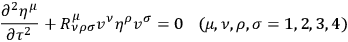
Now the relative motion of free particles is given by the equation of geodesic deviation

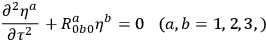
Here is the infinitesimal orthogonal displacement from the (geodesic) worldline of a free particle to that of a neighboring similar particle. is the 4-velocity of the first particle, and the proper time along . If now one introduces an orthonormal frame on , being the timelike vector of the frame, and assumes that the frame is parallelly propagated along (which insures that an observer using this frame will see things in as Newtonian a way as possible) then the equation of geodesic deviation (14.1) becomes

Here are the physical components of the infinitesimal displacement and some of the physical components of the Riemann tensor, referred to the orthonormal frame.

By measurements of the relative accelerations of several different pairs of particles, one may obtain full details about the Riemann tensor. One can thus very easily imagine an experiment for measuring the physical components of the Riemann tensor.

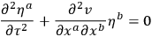
Now the Newtonian equation corresponding to (14.2) is

It is interesting that the empty-space field equations in the Newtonian and general relativity theories take the same form when one recognizes the correspondence between equations (14.2) and (14.3), for the respective empty-space equations may be written and . (Details of this work are in the course of publication in Acta Physica Polonica.)

BONDI: Can one construct in this way an absorber for gravitational energy by inserting a term, to learn what part of the Riemann tensor would be the energy producing one, because it is that part that we want to isolate to study gravitational waves?

PIRANI: I have not put in an absorption term, but I have put in a “spring.” You can invent a system with such a term quite easily.

LICHNEROWICZ: Is it possible to study stability problems for ?

PIRANI: It is the same as the stability problem in classical mechanics, but I haven't tried to see for which kind of Riemann tensor it would blow up.

Interaction of Neutrinos with the Gravitational Field D. Brill

The wave equation of a neutrino in a centrally symmetric gravitational field was derived, using the formalism of Schrödinger and Bargmann. In order to construct a neutrino geon, one must also find the gravitational field produced by a statistical distribution of neutrinos among available states of such a character that the resulting stress energy tensor is spherically symmetric. The stress energy tensor was worked out from a variational principle. The equations which must be solved self-consistently were also worked out for the case of a spherically symmetric neutrino distribution.

BERGMANN: What is the present motivation for the geon research?

WHEELER: The motivation is simply to understand more about how one deals with non-linear field equations. The idea is not that the geon has the slightest to do with an elementary particle, nor with astronomical objects. The interesting things that come out, in the case of the electromagnetic geon, are: if they have any stability at all, and the nature of the radial wave equation for the electromagnetic field. In the neutrino case: first, there is a similarity to the electromagnetic case; second, the radial equation contains a spin orbit coupling term which does not appear in the electromagnetic case, which may help to understand the dynamics of neutrinos.

DE WITT: In this work the neutrinos are not quantized; they are not real neutrinos, are they?

WHEELER: One puts into each neutrino state just one neutrino; this includes all of the results of second quantization.

DE WITT: Might not the gravitational field induce transitions into negative energy states?

WHEELER: This already comes up in the electromagnetic case; what should one use for the stress energy tensor? One counts as gravitation producing only the excitations above the vacuum state, in order to avoid infinities. Here the only neutrino states one considers are the positive energy states; the negative energy states are all filled.

BELINFANTE: You consider a complete absence of antineutrinos; no holes in negative energy states.

WHEELER. Yes, just exactly as one does in the Dirac theory of the electron.

Linear and Toroidal Geons F. J. Ernst

Tolman has shown that there is no gravitational attraction between parallel light rays and that the attraction increases with the angle between the rays, until they are antiparallel. For this reason, a spherical electromagnetic geon is expected to be less stable than a toroidal one. However, the mathematical difficulties in this case are great, and thus as a preliminary step we consider a linear geon, in which the major radius of the toroid has become infinite; we consider light rays travelling along a central axis in both directions. We look for the solution of the coupled equations of general relativity and electromagnetism with a 4-vector potential of a form deduced by analogy with the modes of excitation of a circular wave guide. The equations can then be written down and numerically integrated. One obtains a complete solution of the field equation which contains no singularities. This solution contains an arbitrary constant through which it can be related to the toroidal solution. When the linear geon is bent into torus, this constant is proportional to the major radius.¹

Unified, Non-Symmetrical Field Theory M. Tonnelat

The unified and non-symmetrical field theory starts with a principle which extends the principle of the Born-Infeld electrodynamics. It consists in reducing the sources of the electromagnetic and gravitational field to the field itself.

In order to avoid a point singularity, it is necessary in the static case to define an electric field which is finite at the origin. The formalism of the unified and non-symmetrical field theory immediately introduces the characteristic expressions of Born-Infeld theory.

By writing the fundamental tensor as the sum of two parts, we can relate it to the invariant Lagrangian that appears in the Born-Infeld electrodynamics and the two invariants of the Maxwell theory.

On the other hand, the Einstein theory introduces the contravariant tensor, which may also be written as a sum of symmetric and skew symmetric parts, which shall be called inductions. The relations foreseen partly by the Born-Infeld theory appear between the field and the inductions after making appropriate definitions. The definitions of metric, field and inductions may be chosen in two ways. These definitions depend only on the properties of determinants and on the choice of field and of metric; they do not depend on the Lagrangian of the theory.

We apply the equations of the field to the calculations of a static and spherically symmetric solution of the form chosen by Papapetrou. We can then deduce the radial component of the electrostatic field, . Now introducing like Born-Infeld a field , we set . Then, when approaches 0, approaches , a finite value. The originality of this conclusion comes from the fact that the values of the field and of the metric are not given a priori, but result from the field equations in the particular case of the Schwarzschild solution. We are now led to define a current following the principles of the Born-Infeld theory. We find the charge density, after substitution of the values obtained in the Schwarzschild solution, and upon integrating this over all space, we find the finite value . So from the very principles of the unitary and non-symmetric theory, the distribution of charge is characterized by a “free density” which leads to a finite expression when integrated over the whole space. It is remarkable that this conclusion which results from the Born-Infeld electrodynamics, is connected here with a choice of the fundamental tensor and with an extension of the Schwarzschild solution.

FEYNMAN: How big is for an electron?

TONNELAT: It is exactly like in the Born-Infeld theory; it depends on the choice of ; is a fundamental length. There are two constants of integration which correspond to and mass, but there is a further arbitrariness in the choice of , so that the charge is not determined by the choice of and .

DAVIS: I understand that can be regarded as the ratio of the ordinary electromagnetic field to the natural electromagnetic field. It appears that , as in the Born-Infeld theory could depend on the sign of the charge. Is this correct?

TONNELAT: Yes, appears like the quotient of the physical field and the mathematical field.

Footnotes