Two papers that inaugurated the quantum mechanics of multiparticle systems were published in the second half of 1926. They were “Mehrkörperproblem und Resonanz in der Quantenmechanik” by Werner Heisenberg and “On the Theory of Quantum Mechanics” by Paul Dirac (Heisenberg 1926; Dirac 1926).1 These works are commonly credited together for having laid the foundations of the integration of quantum mechanics and quantum statistics because they introduced the quantum-mechanical expression of the symmetry of a system under exchanges of equal particles. The quantum formalism of exchange symmetry is regarded as having solved at once long-standing difficulties regarding the statistical properties of both equal particles and light quanta by clarifying and legitimizing the previously foggy notion of indistinguishable particles. Despite apparent formal similarities, however, there were significant differences between Heisenberg’s and Dirac’s approaches to multiparticle systems. Furthermore, under the surface of Heisenberg’s distrust of visualizable models and of Dirac’s ideal of abstract theorizing, the two works relied on an interpretive model of particle systems that differed from both earlier and later interpretations of quantum statistics, while remaining surprisingly close to the corpuscular model of the older statistics of James C. Maxwell and Ludwig Boltzmann. Dissonances of this kind are to be expected from two works produced in the early days of quantum mechanics, when the theory was still under construction and questions of interpretation were beginning to surface. One may recall that Max Born’s work on collisions, which opened the way to the statistical interpretation of wave functions, also dates from the summer of 1926. Wolfgang Pauli and Heisenberg formulated the principle of indeterminacy in the following fall and winter. And only in September 1927 did Niels Bohr set forth his principle of complementarity, supposedly providing conceptual unity to the so-called Copenhagen interpretation of quantum mechanics and solving the puzzle of wave-particle duality, under which the interpretation of quantum statistics was filed (Jammer 1966).
While issues of interpretation in quantum mechanics have attracted much historical and philosophical scholarship, the forging of its alliance with quantum statistics remains underexamined. Recent historical analyses have uncovered a plurality of voices under the unisonant narrative of the Copenhagen interpretation, while physical and philosophical work has once again brought to the forefront questions concerning the ontology of quantum mechanics and quantum field theory that were never closed (Beller 1999; Bitbol 2007; Camilleri 2009). Therefore, an investigation of the statistical connections of the early quantum mechanics of multiparticle systems may contribute some clarification. In what follows, I set the stage by recalling the birth of quantum statistics and its first interpretation; then, I analyze Heisenberg’s and Dirac’s pioneering approaches to the integration of quantum statistics and quantum mechanics, with the aim of uncovering the presuppositions of their authors and their interpretations of the outcomes. The purpose is to shed light on the early phase in the historical process of understanding the statistical behavior of multiparticle systems and its connection with the wave-particle duality.
5.1 The Birth of Quantum Statistics
When Heisenberg and Dirac took up the many-particle problem in the emerging framework of quantum mechanics, quantum statistics was itself less than two years old.
It had been born in the second half of 1924, when Albert Einstein applied a statistical method that Satyendra Nath Bose had just worked out for radiation to the ideal gas.
This new theory, which we know as Bose-Einstein statistics, was based on the combinatorial calculation of the entropy of an assembly of “elementary entities”—light quanta or gas molecules—in a quantized phase space.
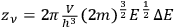
As Einstein explained in the first of his quantum gas papers, the statistical-combinatorial method that Bose had adopted from Max Planck consisted of dividing the phase space of an elementary entity into “cells” of size
 , and defining the “microscopic state” of the assembly as the distribution of the elementary entities over the cells.
Every “macroscopic state” was then assigned a quantity,
, and defining the “microscopic state” of the assembly as the distribution of the elementary entities over the cells.
Every “macroscopic state” was then assigned a quantity,
 , equal to the number of different microscopic states by which the macroscopic state could be thought to be realized.
The quantity
, equal to the number of different microscopic states by which the macroscopic state could be thought to be realized.
The quantity
 was introduced by Planck in his adaptation of Boltzmann’s calculation of the equilibrium distribution of the ideal gas to thermal radiation.
It was used to calculate the entropy,
was introduced by Planck in his adaptation of Boltzmann’s calculation of the equilibrium distribution of the ideal gas to thermal radiation.
It was used to calculate the entropy,
 , and the other thermodynamic functions through the Boltzmann principle,
 . Einstein called it insistently “probability (in Planck’s sense)” or “probability à la Planck,”
evidently to stress that it was no probability in
his sense (Einstein 1924, 261–262; 1925).
There was nonetheless an essential difference between Bose’s calculation and the “quantum statistics” that this method had hitherto produced in the hands of Planck and others.
Einstein compared the two cases in detail in the second of his quantum gas papers, labelling the former method “according to Bose” and the latter “according to the hypothesis of statistical independence of the molecules.”
In both cases, the entropy of a state of the system was proportional to the logarithm of
. Einstein called it insistently “probability (in Planck’s sense)” or “probability à la Planck,”
evidently to stress that it was no probability in
his sense (Einstein 1924, 261–262; 1925).
There was nonetheless an essential difference between Bose’s calculation and the “quantum statistics” that this method had hitherto produced in the hands of Planck and others.
Einstein compared the two cases in detail in the second of his quantum gas papers, labelling the former method “according to Bose” and the latter “according to the hypothesis of statistical independence of the molecules.”
In both cases, the entropy of a state of the system was proportional to the logarithm of
 , which Einstein characterized as the number of “possibilities of realization” of the state.
Likewise, in both cases, a “macroscopically defined state,” or energy distribution, was defined by a set of numbers
, which Einstein characterized as the number of “possibilities of realization” of the state.
Likewise, in both cases, a “macroscopically defined state,” or energy distribution, was defined by a set of numbers
 representing the numbers of elementary entities in each “infinitesimal region” of energy, or “elementary region,”
 .
Finally, within each elementary region, the molecules were to be regarded as distributed among the cells of size
.
Finally, within each elementary region, the molecules were to be regarded as distributed among the cells of size
 in the quantized phase space of a single molecule, and the
 -th elementary region contained
 cells (Einstein 1924, 262).2
Where the two methods differed was in their assumptions of what the “possibilities of realization” of a macroscopic state were.
Though not explicitly defined, these represented a generalization of the configurations of molecules that Boltzmann had named “complexions,” and had to be the most specific states of equal probability by which any other state, as for example an energy distribution, could be thought to be realized.
Indeed, Einstein proceeded to quietly drop the term “possibilities of realization” and to replace it with “microscopically defined states,” while also indicating the term “complexions” in parenthesis.
In the old statistics, the microscopic states were defined by stating “in which cell each molecule sits,” while in the new statistics they were defined by stating
“how many molecules are in each cell” (Einstein 1925, 5–6).
This meant that in the old statistics, one first counted in many different ways how the
cells (Einstein 1924, 262).2
Where the two methods differed was in their assumptions of what the “possibilities of realization” of a macroscopic state were.
Though not explicitly defined, these represented a generalization of the configurations of molecules that Boltzmann had named “complexions,” and had to be the most specific states of equal probability by which any other state, as for example an energy distribution, could be thought to be realized.
Indeed, Einstein proceeded to quietly drop the term “possibilities of realization” and to replace it with “microscopically defined states,” while also indicating the term “complexions” in parenthesis.
In the old statistics, the microscopic states were defined by stating “in which cell each molecule sits,” while in the new statistics they were defined by stating
“how many molecules are in each cell” (Einstein 1925, 5–6).
This meant that in the old statistics, one first counted in many different ways how the
 molecules in the
 -th elementary region could be distributed among the
 phase-space cells of that region.
The result was
phase-space cells of that region.
The result was
 .
Then, one calculated the number of different ways in which the distribution
.
Then, one calculated the number of different ways in which the distribution
 could be obtained from the
 molecules, obtaining the factor
 . Finally, one had to multiply this factor by the product of the
 over all the regions,
 . In the statistics of Bose, the number of ways to partition
 particles into
 cells was given instead by the factor,
 , and the number of complexions corresponding to the energy distribution was given by the product of these factors over all the elementary regions.
The calculation described above was the original form of Einstein’s new statistics.
For the purpose of discussing the integration of quantum statistics with quantum mechanics, however, nothing will be lost if we consider a simpler form, first introduced by Erwin Schrödinger in his examination of Einstein’s quantum gas theory; in this form, the elementary regions of energy are chosen to coincide with the quantum cells (
 ) (Schrödinger 1925).
For the old statistics, then, the number of complexions for a given energy distribution becomes
) (Schrödinger 1925).
For the old statistics, then, the number of complexions for a given energy distribution becomes
 , the factor that Boltzmann used, called “permutability” of the distribution, and from which he derived the Maxwell-Boltzmann distribution.
For the new statistics, the number of complexions becomes equal to one. In the language of quantum atomic theory, which Heisenberg and Dirac used in their treatments of the many-body problem, the change from the Maxwell-Boltzmann statistics to that of Bose and Einstein consisted of the reduction of the statistical weight (Heisenberg’s term), or a priori probability (Dirac’s term), of a state from Boltzmann’s permutability (different for each energy distribution) to one (equal for all the energy distributions).
, the factor that Boltzmann used, called “permutability” of the distribution, and from which he derived the Maxwell-Boltzmann distribution.
For the new statistics, the number of complexions becomes equal to one. In the language of quantum atomic theory, which Heisenberg and Dirac used in their treatments of the many-body problem, the change from the Maxwell-Boltzmann statistics to that of Bose and Einstein consisted of the reduction of the statistical weight (Heisenberg’s term), or a priori probability (Dirac’s term), of a state from Boltzmann’s permutability (different for each energy distribution) to one (equal for all the energy distributions).
Einstein realized that Bose’s way of counting complexions violated an assumption that had, until then, been basic to the statistical method, namely, the statistical independence of the elementary entities. For this reason, he offered Bose’s method as a new statistics alternative to the statistics of independent particles. He made this point very clearly, first in private correspondence and then in the second quantum gas paper (Einstein 1925).3 In his understanding, the new statistics expressed a mutual influence among the elementary entities, which was “for the time being of an entirely mysterious kind” (Einstein 1925, 7). The lack of statistical independence of the light quanta had already been analyzed, especially by Paul Ehrenfest, and Einstein theorized that it was responsible for the wave properties of radiation. For the light quanta, then, the new statistics simply expressed in new form something already known. Einstein surmised that the hypothetical application of the same statistics to the molecules of an ideal gas was justified by a “far reaching formal similarity between radiation and gas,” which he believed to be “more than a mere analogy” (Einstein 1925, 3). He thus suggested that Louis de Broglie’s theory, which attributed wave properties to material corpuscles, might provide the appropriate theoretical framing of the similarity.
Every physicist who commented in print on the new statistics in the two years after its publication adopted Einstein’s interpretation of it as a statistics of non-independence. Schrödinger and Pascual Jordan, however, followed also Einstein’s suggestion of a fundamental similarity between radiation and matter. Schrödinger adopted de Broglie’s ideas and developed them into wave mechanics; Jordan started a treatment of the radiation field that formalized the wave-particle duality within the scheme of the new quantum mechanics (Darrigol 1986; 1992a).
5.2 Heisenberg’s Many-body Problem and Quantum Resonance
The first to find a connection between the quantum mechanics of particles and the new statistics was Heisenberg. Upon accepting the position of lecturer and assistant to Niels Bohr at the Institute of Theoretical Physics in Copenhagen, in April 1926, Heisenberg went to work on the problem of the helium atom. The hypothesis of electron spin that George Uhlenbeck and Samuel Goudsmit put forward in the fall of 1925 had raised hopes to find a common solution for the helium problem and for an explanation of the Pauli Verbot, or “Pauli exclusion rule,” the prohibition of equivalent orbits for atomic electrons postulated by Pauli at the end of 1924. Heisenberg wrote to Pauli at the beginning of May:4
We have found a rather decisive argument that your exclusion of equivalent orbits is connected with the singlet-triplet separation […]. Consider the energy written as a function of the transition probabilities. Then a large difference results if one—at the energy of H atoms—has transitions to 1S, or if, according to your ban, one puts them equal to zero. That is, para- and ortho-[helium] do have different energies, independently of the energies between magnets [i.e., magnetic moments associated with spin].
Heisenberg’s “decisive argument” appeared in Zeitschrift für Physik at the end of June. It was his first published response to wave mechanics, which Schrödinger had just set forth, presenting it as formally equivalent but physically preferable to matrix mechanics. Heisenberg had reacted positively to Schrödinger’s theory, welcoming the formal connection of the two theoretical schemes, and hoping that it might be of help in reaching a physical understanding of quantum mechanics. As he wrote to Dirac:5
I see the real progress made by Schrödinger’s theory in this: that the same mathematical equations can be interpreted as point mechanics in a non-classical kinematics and as wave theory according to Schröd[inger]. I always hope that the solution of the paradoxes in the quantum theory later could be found on this way [sic].
In fact, Heisenberg saw an overthrow of the classical representation of motion in space and time in quantum mechanics, hence a new kinematics, but had been concerned from the onset about the question of how the new kinematics could be understood (Camilleri 2009). Soon, however, he developed a hostility to the physical interpretation that Schrödinger proposed, namely, an open return to a physics of continuous processes in classical space and time. Shortly before submitting his article, Heisenberg wrote to Pauli: “The great achievement of Schrödinger’s theory is the calculation of the matrix elements;” then he added: “The more I ponder the physical part of Schrödinger’s theory, the more horrible I find it.”6 He expressed the same view, in mitigated terms, in the opening of the paper. While acknowledging the convenience of the wave-mechanical approach and its formal connections with the matrix approach, he stressed the difficulties of a wave theory of matter. He closed the introduction stating that, despite the rising of the matter-radiation analogy, “one of the most important aspects of quantum mechanics” was that it was “based upon a corpuscular conception of matter,” even though it was not a description of corpuscles moving in ordinary space and time (Heisenberg 1926, 412). These words echoed the way in which Heisenberg, Born and Jordan had presented matrix mechanics in November 1925. They had described it as “a system of quantum-theoretical relations between observable quantities” which could not be directly interpreted in “a geometrically visualizable way,” because in it the motion of electrons could not “be described in terms of the familiar concepts of space and time” (Born et.al. 1925, 558).
Heisenberg’s strategy for the helium atom was to extend quantum mechanics to a system composed of two electrons coupled by a potential—the simplest example of a many-body system that could model the helium atom—on the basis of an analogy with the classical effect of resonance between two coupled oscillators.
He started by noting that in absence of interaction, the energy of the system was simply the sum of the energies of the two electrons and did not change under the exchange of the two electrons.
He represented the total energy as
 , where
 and
and
 represented the energies of the two electrons, with a and b labelling the electrons, and
 and
and
 their single-electron states.
Correspondingly, he also had distinct states labelled nm and mn in the matrix representing the interaction energy of the system.
Being the electrons perfectly equal particles with identical energy states, the energies of the two states, rather obviously, coincided,
their single-electron states.
Correspondingly, he also had distinct states labelled nm and mn in the matrix representing the interaction energy of the system.
Being the electrons perfectly equal particles with identical energy states, the energies of the two states, rather obviously, coincided,
 . Heisenberg expressed this property by characterizing the energy terms as “twofold”
and then segued into the assertion that the states of the system exhibited what he called “the degeneracy characteristic of the resonance.”
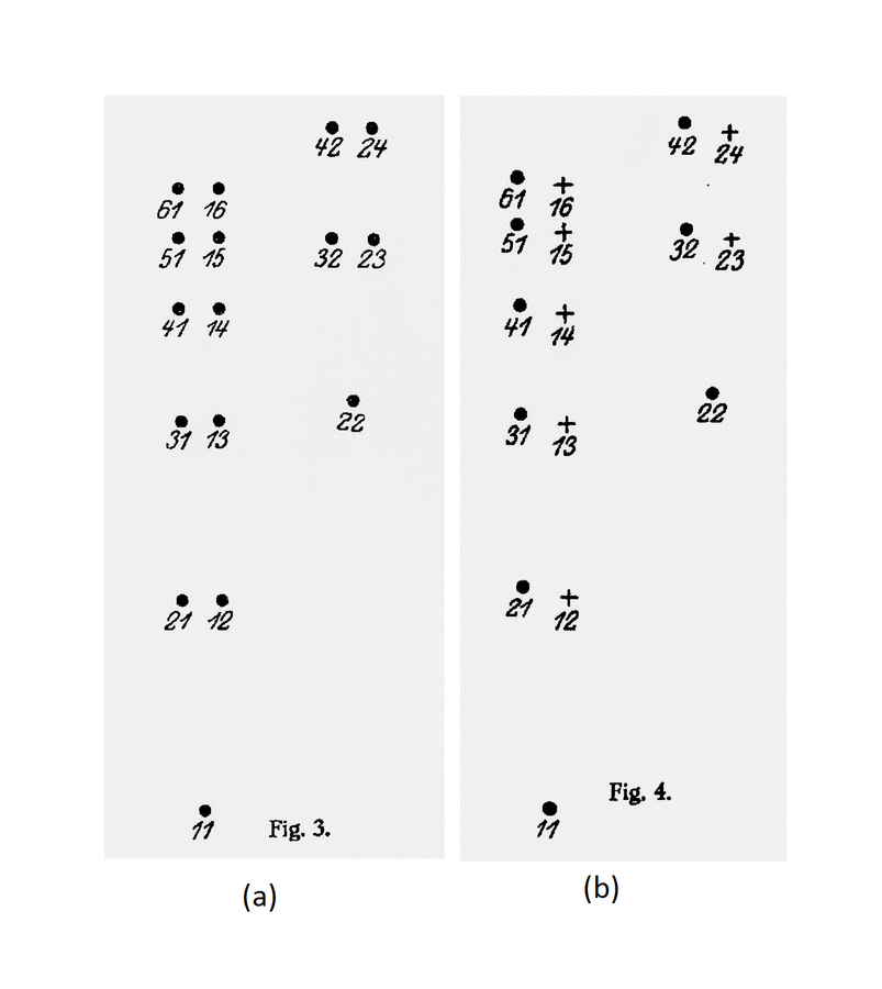
He made the same point graphically, representing the two states separately in a diagram showing the energy levels.
He also admitted, both verbally and graphically, an exception to the twofoldness-degeneracy-resonance, namely, the states in which both electrons had the same energy (fig. 5.1).
Heisenberg did not use too many words to justify his choice to give representation to both states, nm and mn (except for
. Heisenberg expressed this property by characterizing the energy terms as “twofold”
and then segued into the assertion that the states of the system exhibited what he called “the degeneracy characteristic of the resonance.”
He made the same point graphically, representing the two states separately in a diagram showing the energy levels.
He also admitted, both verbally and graphically, an exception to the twofoldness-degeneracy-resonance, namely, the states in which both electrons had the same energy (fig. 5.1).
Heisenberg did not use too many words to justify his choice to give representation to both states, nm and mn (except for
 )
and his identification of twofoldness, degeneracy, and resonance; yet, the choice was neither obvious nor casual, and the identification all but trivial.
As we shall see in the next section, Dirac did pause to ponder how such states should be represented in the matrix form, and made a different choice—ironically, invoking Heisenberg’s methodological principle that the new quantum mechanics should only allow the calculation of observable quantities (Dirac 1926, 666–667). Heisenberg’s priority in dealing with the helium problem was, instead, the expediency of resonance:
)
and his identification of twofoldness, degeneracy, and resonance; yet, the choice was neither obvious nor casual, and the identification all but trivial.
As we shall see in the next section, Dirac did pause to ponder how such states should be represented in the matrix form, and made a different choice—ironically, invoking Heisenberg’s methodological principle that the new quantum mechanics should only allow the calculation of observable quantities (Dirac 1926, 666–667). Heisenberg’s priority in dealing with the helium problem was, instead, the expediency of resonance:
In other words, resonance always occurs when the two systems are not originally in the same state, for the exchange of the two systems gives the same energy. Only in the case of equal energy of the two particles the resonance (or the degeneracy) disappears. (Heisenberg 1926, 417)
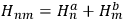
In fact, if an interaction was present and acted as a perturbation on the stationary states of the non-interacting system, there resulted two corrections to the total energy.
Representing with
 the interaction energy, in first approximation the corrections were
 and
and
 .
Each of the twofold energy terms was therefore split into two new values, while no splitting occurred for the terms in which
.
Each of the twofold energy terms was therefore split into two new values, while no splitting occurred for the terms in which
 .
It appears, therefore, that Heisenberg closely followed the analogy with the classical phenomenon of resonance, which was instrumental to the explication of the helium spectrum.
At the same time, he deployed the term “degeneracy” (“Entartung”) from Bohr’s atomic theory, a term that carried a specific assignation of statistical weights, or a priori probabilities.
Bohr’s atomic theory incorporated the rule that every stationary state of an atomic system had the same a priori probability, with the exception of the states that were “degenerate,” that is, they could be adiabatically transformed into two or more states of different quantum energies.
In such cases, Bohr stated that:
.
It appears, therefore, that Heisenberg closely followed the analogy with the classical phenomenon of resonance, which was instrumental to the explication of the helium spectrum.
At the same time, he deployed the term “degeneracy” (“Entartung”) from Bohr’s atomic theory, a term that carried a specific assignation of statistical weights, or a priori probabilities.
Bohr’s atomic theory incorporated the rule that every stationary state of an atomic system had the same a priori probability, with the exception of the states that were “degenerate,” that is, they could be adiabatically transformed into two or more states of different quantum energies.
In such cases, Bohr stated that:
[T]he probability of a given state must be determined from the number of stationary states of some non-degenerate system which will coincide in the given state, if the latter system is continuously transformed into the degenerate system under consideration. (Bohr 1918, 26)
Bohr explicitly crafted his definition of degeneracy to correspond to the classical statistical assumption that a priori probabilities were proportional to volumes in phase space. Along the same lines, Heisenberg took the unperturbed states of the two-electron system to be degenerate or non-degenerate according to whether they were transformed into two new states or into a single one by the interaction. This meant that the assignation of statistical weights was the same as that of any other application of statistical mechanics to quantum systems prior to Bose. Put differently, Heisenberg’s formalism for non-interacting particles channeled exactly the same corpuscular model as the Maxwell-Boltzmann statistics. As we are about to see, Heisenberg was eager to connect his multiparticle quantum mechanics to the new statistics of Bose and Einstein. Nevertheless, his definition of degeneracy for the non-perturbed states reveals that he was not seeking the connection because he had come to a reexamination of the nature of particles in the light of the new kinematics.
In accord with his application of Bohr’s rule, Heisenberg further asserted that the degeneracy was “eliminated in the system perturbed by the interaction” (Heisenberg 1926, 417). He also warned, however, that although he continued to label the new states nm and mn, the indices no longer referred to the states of the individual particles. He further warned that it no longer made “physical sense to talk” about the motion of single electrons (Heisenberg 1926, 418, 423).
Thus, he arrived at what he regarded as the decisive result.
Because of the equality of the two electrons, the matrix representing the radiation emitted by the system had to be symmetric under electron exchanges.
This requirement entailed that the new energy levels divided into two sets (which Heisenberg marked with the symbols
 and
and
 , see fig. 5.1), such that the amplitudes of all the transitions from the energy levels of one set to those of the other set were zero.
No transition would occur from one set to the other; as Heisenberg put it, the two sets could “in no way combine with each other” (Heisenberg 1926, 418). Resonance produced, therefore, an indeterminacy in the possible solutions of the problem. Either one of the two sets of terms, as well as a mixture of the two, constituted a complete solution, and the theory alone could not decide which choice was correct.
, see fig. 5.1), such that the amplitudes of all the transitions from the energy levels of one set to those of the other set were zero.
No transition would occur from one set to the other; as Heisenberg put it, the two sets could “in no way combine with each other” (Heisenberg 1926, 418). Resonance produced, therefore, an indeterminacy in the possible solutions of the problem. Either one of the two sets of terms, as well as a mixture of the two, constituted a complete solution, and the theory alone could not decide which choice was correct.
At this point, Heisenberg examined the problem through Schödinger’s formalism.
Applying the relations between matrix elements and eigenfunctions, he found that the eigenfunctions of the perturbed system were the two linear combinations of single-electron eigenfunctions.
Indicating with
 and
and
 the eigenfunctions of the two electrons,
 and
and
 , in the unperturbed single-electron energy states of energies
 and
and
 , the eigenfunctions of the whole system in the perturbed case were
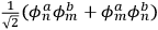 and
and
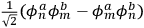 (Heisenberg 1926, 420).
 and
and
 . Source: (Heisenberg 1926, 417–418).
Fig. 5.1: Heisenberg’s diagrams illustrating the states of a system of two electrons. (a) Without interaction, every energy value is twofold or degenerate, except when the electrons are in the same single-electron state. (b) With interaction, the degeneracy is broken, and the states divide into two non-combining sets, indicated by
and
. Source: (Heisenberg 1926, 417–418).
Heisenberg was then able to show that the predicted phenomenon of quantum resonance could reproduce, qualitatively and in order of magnitude, the spectrum of helium. The Coulomb repulsion between the two electrons of the helium atom would cause a “large electrical resonance,” and the corresponding energy separation between the two sets reproduced in order of magnitude the differences between the spectra of ortho-helium and para-helium. If then the electrons were regarded as “small magnetic spinning tops,” the large resonance would be perturbed. On the one hand, weak transitions between the two sets would now be permitted thanks to “the interaction between magnet and orbit.” However, each stationary state would become fourfold (there would be four possible combinations of the two spins), and a “finer exact resonance” would occur on account of the interaction between spins, which would again produce a separation into two non-combining sets (Heisenberg 1926, 421–422). Heisenberg then observed that of the two theoretically possible sets of terms, only one agreed with experiment, namely, the one in which there were no equivalent orbits and in which, therefore, the Pauli Verbot was satisfied. Although he could not find a reason why only one of the two sets should be selected, he was at least able to offer a formal representation of the empirical rule.
In the last section of the paper Heisenberg made the connection with Bose-Einstein statistics. In a swoop of guesswork, he argued that if his results were generalized to an arbitrary number of electrons, it then became possible to use the indeterminacy of the stationary states and the Pauli rule to deduce the statistics of the assembly. According to him, the selection of only one of the theoretically possible solutions according to the now-formalized Pauli rule would result in a “reduction of the statistical weights” of the states that corresponded precisely to “the Bose-Einstein counting” (Heisenberg 1926, 422). He claimed that this formulation of the new assignation of statistical weights surpassed Einstein’s, for it not only prescribed the choice of one specific solution out of many, it also specified the right choice, because it demanded the one set that satisfied the Pauli Verbot.
Heisenberg counted this outcome as a success. Even though he could not justify the natural selection of a single solution, having found a formal scheme that simultaneously reproduced the Pauli rule and the Bose-Einstein statistics was nonetheless an important result, since it indicated that they had the same cause. He recalled that an interaction was necessary among the particles for the quantum-mechanical resonance to occur, but he did not care to clarify what this meant for the molecules of the Bose-Einstein ideal gas. He also emphasized that the theoretical success came at a cost: it no longer made “physical sense to talk of” the motion of single electrons (Heisenberg 1926, 423). This startling restriction went beyond the notion that the theory described individual corpuscles in non-ordinary space and time. Heisenberg, however, defused its ontological potential by asserting that it made no sense to speak of the motion of individual electrons just as it made no sense to speak of any non-symmetrical function of the electrons, because only symmetric functions represented observable quantities. Finally, he returned to the wave interpretation to conclude that it could now be dismissed. Not only did the corpuscular interpretation alone suffice to deal with multiparticle systems, it even afforded a smooth integration of quantum mechanics with the statistical theory that had seemed to support the undulatory conception of matter.
Despite his assurance, in the statistical part of the argument, Heisenberg was flying by the seat of his pants.
Most blatantly, he did not recognize that the Bose-Einstein statistics, in which there was no restriction on the number of particles allowed in a state, was incompatible with the Pauli Verbot, which allowed no more than one particle in each state.
A few months earlier, Enrico Fermi had published a new quantum statistics of the ideal gas that was explicitly based on the generalization of the Pauli rule (Fermi 1926, reprinted in: Amaldi et.al. 1962, 181–185).
Fermi, a young theorist in Rome who was not yet a member of the quantum network, had worked within the framework of the old quantum mechanics.
Dirac would shortly arrive at the same quantum statistics in his treatment of many-particle systems in quantum mechanics.
Heisenberg, who was evidently unaware of Fermi’s work, confused the two quantum statistics, and strangely continued to confuse them even after the publication of Dirac’s paper.
This oversight was not the only peculiarity of Heisenberg’s argument, however.
In his reckless generalization from two to
 electrons, Heisenberg took the Bose-Einstein statistics to amount to a “reduction of statistical weights from
 to 1” (Heisenberg 1926, 423).
But the statistical weight assigned by the old statistics to a macroscopic state was not
to 1” (Heisenberg 1926, 423).
But the statistical weight assigned by the old statistics to a macroscopic state was not
 .
It was Boltzmann’s permutability,
.
It was Boltzmann’s permutability,
 , as we have seen in the previous section.
Next, Heisenberg assumed that every energy value of the unperturbed
, as we have seen in the previous section.
Next, Heisenberg assumed that every energy value of the unperturbed
 -particle system was
 -fold degenerate, even though he had denied earlier that this was always the case.
The states
-fold degenerate, even though he had denied earlier that this was always the case.
The states
 and
and
 , for instance, were non-degenerate in his scheme (fig. 5.1).
Therefore, according to his reasoning, the degeneracy factor should again have been the permutability, not the number of particle permutations,
, for instance, were non-degenerate in his scheme (fig. 5.1).
Therefore, according to his reasoning, the degeneracy factor should again have been the permutability, not the number of particle permutations,
 .
That replacement of the permutability with the factorial of
.
That replacement of the permutability with the factorial of
 was a standard approximation in statistical calculations, in which it was often possible to assume that the frequency of cases of particles of equal energies was negligible, may partly account for Heisenberg’s slip; still, the replacement was indefensible in the case of an atomic system.
Although these twin inaccuracies neutralized one another as far as Heisenberg’s aim was concerned, they had the unfortunate effect of masking the actual difference between the old and the new statistics.
A simple reduction of statistical weights by a common factor, such as Heisenberg implied, would have left the statistical distribution of macrostates unchanged.
Furthermore, Heisenberg went on to claim that quantum resonance caused, quite conveniently, a separation into precisely
was a standard approximation in statistical calculations, in which it was often possible to assume that the frequency of cases of particles of equal energies was negligible, may partly account for Heisenberg’s slip; still, the replacement was indefensible in the case of an atomic system.
Although these twin inaccuracies neutralized one another as far as Heisenberg’s aim was concerned, they had the unfortunate effect of masking the actual difference between the old and the new statistics.
A simple reduction of statistical weights by a common factor, such as Heisenberg implied, would have left the statistical distribution of macrostates unchanged.
Furthermore, Heisenberg went on to claim that quantum resonance caused, quite conveniently, a separation into precisely
 non-combining sets of states.
He was unable to prove the claim, and in less than six months, Eugene Wigner dismantled it.
Through a careful examination of a system of three interacting particles, Wigner showed that the separation into non-combining sets did occur, but the number of non-combining sets was only three.
To handle the problem for higher values of
non-combining sets of states.
He was unable to prove the claim, and in less than six months, Eugene Wigner dismantled it.
Through a careful examination of a system of three interacting particles, Wigner showed that the separation into non-combining sets did occur, but the number of non-combining sets was only three.
To handle the problem for higher values of
 , one needed the mathematical theory of groups, and the solution did not turn out to be
 (Wigner 1927a; 1927b). Finally, Heisenberg oddly insisted that the reduction of statistical weights was caused by “the choice of one quantum mechanical solution out of many possible solutions,” even though according to Bohr's rule the reduction was effected simply by the removal of degeneracy (Heisenberg 1926, 425).
Why did Heisenberg get himself into this jumble?
To recover the Bose-Einstein statistics, it would have been sufficient to generalize Bohr’s rule by assuming that all the possible perturbed multiparticle states had the same statistical weight.
Dirac was to take this route, as we shall see.
The reason for the unnecessary complication of Heisenberg’s argument may reside in the incompleteness of his interpretation of the formalism, and in the ambiguity in which it left the ontological status of multiparticle states.
Heisenberg was careful not to pronounce himself too finely on ontology beyond his advocacy of the corpuscular interpretation and his rejection of classical kinematics. Nevertheless, his apparent fondness of the number
 suggests that his heuristic resource for theory construction was still the classical conception of an assembly of free particles.
He regarded every energy value of the free-particle system as degenerate because it was potentially obtainable in multiple ways through exchanges of equal particles.
For two particles, this classical notion accorded with Bohr’s definition of degeneracy, and Heisenberg rashly assumed that the accord would persist for any number of particles.
Since he considered every multiparticle state as degenerate, he assigned it a statistical weight equal to
suggests that his heuristic resource for theory construction was still the classical conception of an assembly of free particles.
He regarded every energy value of the free-particle system as degenerate because it was potentially obtainable in multiple ways through exchanges of equal particles.
For two particles, this classical notion accorded with Bohr’s definition of degeneracy, and Heisenberg rashly assumed that the accord would persist for any number of particles.
Since he considered every multiparticle state as degenerate, he assigned it a statistical weight equal to
 , that is, the number of possible particle permutations, easily forgetting the anomaly presented by particles of equal energy.
But what happened to the supposed degeneracy when an interaction deprived the particles of their freedom?
The self-imposed prohibition to talk of individual corpuscles moving in ordinary space and time deprived Heisenberg of the possibility to interrogate the classical corpuscular model, while it did not itself provide an answer.
In these circumstances, the formalism was mute.
It is probably in order to resolve the ambiguity that Heisenberg reached for a mechanism capable of suppressing any potential degeneracy, and the Pauli-rule selection, albeit unjustified, seemed to him suitable to this purpose.
, that is, the number of possible particle permutations, easily forgetting the anomaly presented by particles of equal energy.
But what happened to the supposed degeneracy when an interaction deprived the particles of their freedom?
The self-imposed prohibition to talk of individual corpuscles moving in ordinary space and time deprived Heisenberg of the possibility to interrogate the classical corpuscular model, while it did not itself provide an answer.
In these circumstances, the formalism was mute.
It is probably in order to resolve the ambiguity that Heisenberg reached for a mechanism capable of suppressing any potential degeneracy, and the Pauli-rule selection, albeit unjustified, seemed to him suitable to this purpose.
That Heisenberg’s treatment of the many-body problem was informed by the classical model of particle assemblies is also supported by the few explicit remarks that he made concerning the interpretation of the formalism. From the viewpoint of the corpuscular interpretation, the perturbed energies contained terms corresponding to “transitions in which the electrons exchange[d] place” (Heisenberg 1926, 417). Therefore, Heisenberg explained that in each perturbed state the electrons had “the same motion (in different phases)” (Heisenberg 1926, 418). He regarded this effect as the analog of classical resonance between coupled oscillators. While he declared that in presence of an interaction it no longer made “physical sense to talk of” the motion of single electrons, he also advised that if you wanted to form a picture of the motions, you could imagine the electrons to “exchange place periodically in a continuous way” (Heisenberg 1926, 421 and 423).7
5.3 Dirac’s “On the Theory of Quantum Mechanics”
The second treatment of many-particles systems in quantum mechanics was given shortly thereafter by Dirac in a paper titled “On the Theory of Quantum Mechanics” (Dirac 1926). As for Heisenberg, this was also Dirac’s first published response to Schrödinger’s theory. He had corresponded with Heisenberg while completing his PhD thesis in Cambridge in the spring of 1926. Many years later, he wrote in his recollections that he did the work on many-particle systems after Heisenberg convinced him of the usefulness of wave mechanics. Dirac felt “at first a bit hostile” to this theory because it seemed to him that it represented a regress to “the pre-Heisenberg stage.” In a non-extant letter to Heisenberg, he criticized Schrödinger because “the wave theory of matter must be inconsistent just like the wave theory of light” (Dirac 1977, 131–132). Heisenberg agreed with this criticism but nonetheless saw Schrödinger’s theory as progress, as we have seen. Thanks to Heisenberg’s detailed explanation of the relation between the two formal schemes, Dirac could see that wave mechanics “would not require us to unlearn anything that we had learned from matrix mechanics” but rather “supplemented the matrix mechanics and provided very powerful mathematical developments which fitted perfectly with the ideas of matrix mechanics” (Dirac 1977, 133).
In Dirac’s retrospective account, it was the study of Schrödinger’s formalism that suggested to him the possibility of symmetric and antisymmetric wave functions for a system of similar particles. These “symmetry questions,” in turn, “brought in the possibility of new laws of Nature” (Dirac 1977, 133). But the inspiration to explore the symmetry of the wave functions might not have been as purely formalistic as it appeared to Dirac in hindsight. In fact, Dirac knew that Heisenberg was working on the helium atom, because Heisenberg had written to him of his idea that the explanation of the helium spectrum was “a resonance effect of a typical quantum mechanical nature.”8 Moreover, in an “added in proof” footnote in his paper, Dirac wrote: “Prof. Born has informed me that Heisenberg has independently obtained results equivalent to these” (Dirac 1926, 670). Dirac probably met Born in late July, when the latter was in Cambridge to give a talk at the Kapitza Club (Kragh 1990, 321, note 68; Darrigol 1992b). Therefore, he knew about Born’s thoughts on the superposition of wave functions, and it is also likely that he learned about Heisenberg’s results before submitting his paper in late August. Nevertheless, Dirac proceeded differently from Heisenberg and he also reached significantly different results.
Instead of confronting Schrödinger’s undulatory interpretation, Dirac set out to reformulate Schrödinger’s formal apparatus in general terms according to his own mathematical approach. He deduced the expression of the general solution of a quantum-mechanical problem as a linear expansion with arbitrary constants in “a set of independent solutions,” which he called eigenfunctions (Dirac 1926, 664). This formal milestone enabled him to develop a quantum-mechanical treatment of multiparticle systems and to reach three lasting results. He arrived at the symmetry and antisymmetry of the wave functions, formulated the statistics that we now know as Fermi-Dirac statistics, and derived a calculation of Einstein’s coefficients of absorption and stimulated emission. While Heisenberg welcomed the wave theory because it showed that the mathematical apparatus could be interpreted in two ways, Dirac adopted the wave formalism as an enhanced mathematical apparatus from which it was possible to calculate the matrices of the older formulation. He believed that questions of interpretation should be broached only after a general formal scheme was developed as abstractly as possible (Darrigol 1992b). Nonetheless, since he did need an interpretive model to extend the formalism to a new kind of physical system, he openly relied on the interpretation of the matrices in terms of particles and quantum transitions, simply sidestepping the wave aspects of the theory.
As Heisenberg, Dirac adopted “an atom with two electrons” as the simplest multiparticle system. In his atom, however, all interactions between electrons could be neglected. He did not resort to the analogy with the classical phenomenon of resonance as a theoretical tool, but used only the symmetry of the two-electron system supplemented by the methodological principle for which he credited Heisenberg:
[Heisenberg’s matrix mechanics] enables one to calculate just those quantities that are of physical importance, and gives no information about quantities such as orbital frequencies that one can never hope to measure experimentally. We should expect this very satisfactory characteristic to persist in all future developments of the theory. (Dirac 1926, 667)
Dirac indicated with
 “the state of the atom in which one electron is in an orbit labelled
 and the other in the orbit
 .”
He then asked the question that Heisenberg had not considered worth asking.
Were the “physically indistinguishable” states
.”
He then asked the question that Heisenberg had not considered worth asking.
Were the “physically indistinguishable” states
 and
and
 to be counted as distinct or as identical? This question was inconsequential in classical mechanics, but in the matrix formalism, it implied a choice between two different matrix representations. In one, the matrix elements corresponding to the transitions
 and
and
 would be represented by two separate matrix elements, in the other they would be represented by the same element.
In principle, Dirac could have relied on the traditional statistics of particles to answer the question; in that case, the answer would have been that the two states were distinct except when
would be represented by two separate matrix elements, in the other they would be represented by the same element.
In principle, Dirac could have relied on the traditional statistics of particles to answer the question; in that case, the answer would have been that the two states were distinct except when
 .
In the previous section, we saw that Heisenberg had taken this course in his treatment of the helium atom. He had simply adopted the first representation and had applied symmetry considerations only to the values of the matrix elements representing the radiation emitted and absorbed by the system of interacting particles, thereby deducing the impossibility of transitions between two groups of terms.
Dirac, who possibly had learned from Born of Heisenberg’s linkage of quantum mechanics and Bose-Einstein statistics, instead chose to ignore the prescription of the old statistics. He asserted that the two transitions,
.
In the previous section, we saw that Heisenberg had taken this course in his treatment of the helium atom. He had simply adopted the first representation and had applied symmetry considerations only to the values of the matrix elements representing the radiation emitted and absorbed by the system of interacting particles, thereby deducing the impossibility of transitions between two groups of terms.
Dirac, who possibly had learned from Born of Heisenberg’s linkage of quantum mechanics and Bose-Einstein statistics, instead chose to ignore the prescription of the old statistics. He asserted that the two transitions,
 and
and
 , were “physically indistinguishable” and that “only the sum of the intensities for the two together could be determined experimentally” (Dirac 1926, 667). From this proposition he drew the answer:
Hence, in order to keep the essential characteristic of the theory that it shall enable one to calculate only observable quantities, one must adopt the second alternative thatand
count as only one state. (Dirac 1926, 667)
Having so fixed the matrix formalism, Dirac applied his formula for the general solution of the two-particle model. He formed the eigenfunctions of the whole system as linear combinations of products of the eigenfunctions of the single electrons; then, he imposed the condition that they correspond to the matrices. This condition could be satisfied only by combinations that were symmetrical or antisymmetrical under exchange of the electrons. Either one of these two possibilities gave “a complete solution of the problem” and quantum mechanics did not dictate which was the correct one (Dirac 1926, 669). The choice, Dirac stated, was to be made by appealing to Pauli’s exclusion principle:
An antisymmetrical eigenfunction vanishes identically when two of the electrons are in the same orbit. This means that in the solution of the problem with antisymmetrical eigenfunctions there can be no stationary states with two or more electrons in the same orbit, which is just Pauli’s exclusion principle. (Dirac 1926, 669–670)
The symmetrical solution, however, could not be correct for “the problem of electrons in an atom” because it allowed any number of electrons in the same orbit (Dirac 1926, 670). These results could be straightforwardly extended to any system composed of similar particles, in particular, to an assembly of molecules. Dirac thus applied them to the ideal gas. He obtained the eigenfunction of the assembly by multiplying the single-molecule eigenfunctions and choosing either the symmetrical or the antisymmetrical linear combinations. At this point, he turned to statistical considerations. He implicitly made the assumption that the new states, represented by symmetrical and antisymmetrical wavefunctions, represented the energy distributions, or macrostates, of statistics. Then, he explicitly adopted as a “new assumption” the simplest extension of Bohr’s rule, namely, that “all the stationary states of the assembly (each represented by one eigenfunction) have the same a priori probability” (Dirac 1926, 671). In the case of symmetrical eigenfunctions, this rule corresponded to the Bose-Einstein statistics. In the case of the antisymmetrical eigenfunctions, whereby the number of molecules associated with each single-particle eigenfunction could only be 0 or 1, it led to the new statistics that is now known as the Fermi-Dirac statistics. Dirac concluded:
The solution with symmetrical eigenfunctions must be the correct one when applied to light quanta, since it is known that the Einstein-Bose statistical mechanics leads to Planck’s law of black-body radiation. The solution with antisymmetrical eigenfunctions, though, is probably the correct one for gas molecules, since it is known to be the correct one for electrons in an atom, and one would expect molecules to resemble electrons more closely than light quanta. (Dirac 1926, 672)
Despite having just derived the two quantum statistics from the same set of assumptions (with the difference of the Pauli principle), Dirac separated them starkly in their applicability. His integration of quantum statistics and quantum mechanics was thus sealed with an uncompromising rejection of Einstein’s analogy between light quanta and material corpuscles. Dirac, in fact, had already rejected the matter-radiation analogy two years earlier:
For the discussion of equilibrium problems, quanta of radiation cannot be regarded as very small particles moving with very nearly the speed of light. There are two important points in which this picture is inadequate. In the first place the small particles could not (according to ordinary statistical theory) have any stimulating effect on processes by which they are emitted, and they should therefore be distributed in momentum according to Maxwell’s law, which is the same as being distributed in energy (or frequency) according to Wien’s radiation law. Secondly the concentration of quanta in thermodynamical equilibrium is not arbitrary, as is the case with all kinds of material particles, but is a definite function of temperature. (Dirac 1924, 594)
Moreover, when he first studied Einstein’s quantum gas theory, he followed Einstein’s interpretation of Bose’s method as a statistics of non-independent entities. If the gas molecules were statistically distributed as light quanta, then they would have to be “not distributed independently from one another,” and hence there would have to be “some kind of interaction between them” (Dirac 1925, 7). For Dirac, therefore, the analogy of ideal gas and heat radiation was invalid because non-interacting molecules had to be statistically independent, while light quanta were known not to be so. His categorical separation of the domains of applicability of the two quantum statistics preempted the possibility to interpret his new statistics in the same way as the statistics of Einstein and Bose, that is, as a statistics of non-independence.
A retrospective comparison with the modern understanding of quantum statistics brings into relief what Dirac’s argument was not about. He did not argue that his formal-observational symmetry signified any modification of the traditional model of particles. More specifically, he did not propose that in the new mechanics, the particles were any more indistinguishable than they already were in classical mechanics. He did not suggest that the particles lost their identity. He flatly ignored the possibility that they had wave-like properties. Finally, he did not even extend the interpretation of the Bose-Einstein statistics as a statistics of non-independent objects to his new statistics. The only implication that he drew from his implementation of the formal-observational symmetry was a confirmation of the fundamental difference between material particles (electrons, atoms and molecules) and light quanta.
Dirac’s integration of quantum statistics and quantum mechanics rested squarely on the corpuscular interpretation of the matrix formalism, supplemented by a formal restriction on the solutions of the wave equation.
Dirac justified the formal restriction in terms of observational symmetry. Planck had already invoked the symmetry of a gas under exchanges of equal molecules in the quantum-statistical theory of gas prior to Bose.
He and others used it to rationalize the subtraction of a term depending on the number of particles from the expression of the entropy (Darrigol 1991; Desalvo 1992; Monaldi 2009).
Schrödinger had compared the entropy formula obtained in this way with the formula derived by Einstein, and he had concluded that the correct implementation of Planck’s exchange symmetry was the statistics of non-independence proposed by Einstein.
He then floated the suggestion that the proper way to understand this odd new statistics might be to regard the whole gas as a system endowed with a “symmetry number” equal to
 rather than as an assembly of
 independent individual molecules (Schrödinger 1925, 438).
Therefore, a viable, if still sketchy, model based on exchange symmetry was available to Dirac to support his symmetry requirement.
Nonetheless, he was clear and explicit that for him the state
independent individual molecules (Schrödinger 1925, 438).
Therefore, a viable, if still sketchy, model based on exchange symmetry was available to Dirac to support his symmetry requirement.
Nonetheless, he was clear and explicit that for him the state
 was not an unspecific state of the whole system endowed with symmetry, but a state “in which one electron is in an orbit labelled
 , and the other in the orbit
 ” (Dirac 1926, 667).
In other words, Dirac remained faithful to the individuality of particles typical of the corpuscular interpretation of matrix mechanics, skirting the implications of his new statistics for the independence of electrons and gas molecules.
” (Dirac 1926, 667).
In other words, Dirac remained faithful to the individuality of particles typical of the corpuscular interpretation of matrix mechanics, skirting the implications of his new statistics for the independence of electrons and gas molecules.
The fact that Dirac disregarded the undulatory interpretation of the wave function and the consequences of antisymmetry for the independence of material particles does not mean that he refrained completely from any interpretation of the general solution of the wave equation.
He did put forward an interpretation in the last section of the paper, in which he outlined a perturbation theory and fruitfully put it to use.
He wrote the wave equation of “an atomic system subjected to a perturbation from outside (e.g., an incident electromagnetic field),” and showed that the general solution could be written as
 , where the
 were the wave functions associated with the stationary states of the unperturbed atom, and the
 coefficients depending on time.
He thus deftly switched interpretive models.
He proceeded to consider the general solution as no longer representing an atom but an assembly of atoms, and to assume that the square modulus of the coefficient
coefficients depending on time.
He thus deftly switched interpretive models.
He proceeded to consider the general solution as no longer representing an atom but an assembly of atoms, and to assume that the square modulus of the coefficient
 represented “the number of atoms in the
 th state” (Dirac 1926, 646–647).
The general solution now was a new theoretical representation of a multiparticle system that avoided any representation of individual particles and therefore bypassed, for the time being, the question of whether two states differing only by particle exchange should be counted as a distinct or identical.
Determining the time evolution of the
th state” (Dirac 1926, 646–647).
The general solution now was a new theoretical representation of a multiparticle system that avoided any representation of individual particles and therefore bypassed, for the time being, the question of whether two states differing only by particle exchange should be counted as a distinct or identical.
Determining the time evolution of the
 under the effect of the perturbation, Dirac was then able to derive the coefficients of absorption and stimulated emission of Einstein’s theory of radiation, under the restricting condition that the initial phases of the atoms could be averaged.
In this part of the paper, Dirac made no use of the results of the previous section.
Neither did he subject the assembly of atoms to the exclusion principle that he had just posited to apply to gas molecules, nor did he suppose that the atoms followed the Einstein-Bose statistics.
under the effect of the perturbation, Dirac was then able to derive the coefficients of absorption and stimulated emission of Einstein’s theory of radiation, under the restricting condition that the initial phases of the atoms could be averaged.
In this part of the paper, Dirac made no use of the results of the previous section.
Neither did he subject the assembly of atoms to the exclusion principle that he had just posited to apply to gas molecules, nor did he suppose that the atoms followed the Einstein-Bose statistics.
Dirac returned to the difference between electrons and light quanta and the emission and absorption of radiation half a year later, after having spent several months at Bohr’s institute in Copenhagen formulating the general transformation theory and a general statistical interpretation of it (Dirac 1977; Kragh 1990; Darrigol 1992b). As a result of that work, he was able to forge a link between his two representations of multiparticle systems for the case of light quanta, and thereby launched quantum electrodynamics. He first provided a quantum-mechanical theory of the radiation field using the energies and phases of the Fourier components as dynamical variables. Then, adapting his earlier tentative interpretation of the general solution of the wave equation, and helping himself with some nimble assumptions, he built a formal equivalence between the Hamiltonian of the field and the Hamiltonian of an assembly of equal particles (Darrigol 1986; Schweber 1994). He stressed, however, that the equivalence worked only if the particles obeyed the Bose-Einstein statistics, and this meant that it could only work for light quanta. Although Dirac now enlarged the term “particles” to include these entities, it was clear that for him they still did not belong in the same category as electrons. He especially warned that the classical “light wave” did not coincide with the “de Broglie or Schrödinger wave associated with the light quanta.” Therefore, even though there was a “de Broglie or Schrödinger wave” associated with each electron, there could not be a corresponding field description for electrons with them (Dirac 1927, 241).
In addition, Dirac now had at his disposal the statistical interpretation of the theory. He was therefore able to reaffirm the connection between symmetric wave functions and Bose-Einstein statistics without the need for an additional assumption concerning the equal probabilities of the stationary states. He pointed out that the wave function of an assembly of particles could now be interpreted “in the usual manner.” By this, he meant that the wave function no longer gave “merely the probable number” of particles in any state, but gave also “the probability of any given distribution” of the particles over the various states. But the probability calculated in this way did not agree with the probability calculated “from elementary considerations” for an assembly of independent particles. It agreed with the probability of an assembly of particles that obeyed the Bose-Einstein statistics, thus confirming the latter as a statistics of non-independence. In spite of the generality of the statistical interpretation, Dirac neglected to extend the same conclusion to the Fermi-Dirac statistics (Dirac 1927, 251). For a time, he continued to regard the two statistics as revealing two fundamentally different ontologies. As he recalled in his memoir, at first he disliked Jordan and Wigner’s extension of his field quantization technique to particles obeying the Fermi-Dirac statistics. His objection was that in the case of Bose-Einstein statistics, one could form “a definite picture underlying the basic equations, namely the picture that the theory could be applied to an assembly of oscillators.” No corresponding picture was available for the Fermi-Dirac statistics, and Dirac felt that this “was a serious drawback” (Dirac 1977, 140).
5.4 Conclusion
Despite their similarities, the works of Heisenberg and Dirac on the quantum mechanics of multiparticle systems present significant differences. Heisenberg was driven by the need to solve the problem of the helium atom and by the antagonism between his corpuscular interpretation and Schrödinger’s undulatory interpretation of quantum mechanics. He relied on the phenomenon of quantum resonance, for which an interaction among the particles was necessary. Although he discarded classical kinematics, he took for granted that two states of free particles that differed only by particle exchange should be represented as distinct, except for the cases in which the particles had the same energy. He mistook the Bose-Einstein statistics for a statistics compatible with Pauli’s exclusion principle, and he saw the transition from the old to the new statistics as the effect of a splitting of the energy states caused by resonance plus the natural selection of the single set of states that verified the exclusion principle. Dirac, in contrast, sidestepped the wave model and was mainly motivated by his mathematical reformulation of the wave formalism. Neglecting all interactions among the particles, he relied mainly on the symmetry of a system of equal particles and on the metatheoretical precondition that the theory yield only observable quantities. On this basis, contrary to Heisenberg, he concluded that two states differing only by particle exchange should be represented as a single state. This led him to the requirement of either symmetrical or antisymmetrical stationary states. He could then relate the symmetrical states to the Bose-Einstein statistics, and the antisymmetrical states to the exclusion principle and to the Fermi-Dirac statistics. Unlike Heisenberg, Dirac drew a categorical distinction between material corpuscles, all of which in his view followed the Fermi-Dirac statistics, and light quanta, which followed instead the Bose-Einstein statistics.
The comparison also brings to light a deeper commonality. Although these two papers played a prominent role in the interaction of quantum statistics and wave-particle duality, neither of them was produced on the basis of a revision of the traditional concept of particles. On the contrary, they both reveal a firm reliance on the corpuscular interpretive model, which continued to dominate the theoretical imagination of the two theorists, notwithstanding their overthrow of the classical representation of motion and their formalistic stances. Heisenberg’s traditional assignation of statistical weights within the context of quantum mechanics and Dirac’s drastic separation of the two quantum statistics can be seen as symptomatic of a remarkable theoretical resilience of the corpuscular model. More specifically, they point to the relative autonomy and persistence across theory changes of two basic characteristics of the concept of individual particles, their perfect similarity and their mutual statistical independence.
Abbreviations and Archives
| AHQP | Archive for History of Quantum Physics. American Philosophical Society, Philadelphia |
| Einstein Archives | Hebrew University of Jerusalem |
References
Amaldi, Edoardo, Enrico Persico, E. P., Rasetti Enrico (1962). Enrico Fermi. Collected Papers (Note e Memorie). Vol. 1. . Chicago: The University of Chicago Press.
Beller, Mara (1999). Quantum Dialogue: The Making of a Revolution. Chicago: The University of Chicago Press.
Bitbol, Michel (2007). Schrödinger against Particles and Quantum Jumps. In: Quantum Mechanics at the Crossroads: New Physics, Novel Historical and Philosophical Views Ed. by James Evans, Alan S. Thorndike. Berlin: Springer 81-100
Bohr, Niels (1918). On the Quantum Theory of Line Spectra. In: Det Kongelige Danske Videnskabernes Selskab. Skrifter. Naturvidenskabelig og Matematisk Afdeling, Part 1 1-36
Born, Max, Werner Heisenberg, W. H. (1925). Zur Quantenmechanik II. Zeitschrift für Physik 35: 557-615
Camilleri, Kristian (2009). Heisenberg and the Interpretation of Quantum Mechanics. The Physicist as Philosopher. Cambridge: Cambridge University Press.
Carson, Cathryn (1996). The Peculiar Notion of Exchange Forces—I. Origins in Quantum Mechanics, 1926–1928. Studies in History and Philosophy of Modern Physics 27: 23-45
Darrigol, Olivier (1986). The Origin of Quantized Matter Waves. Historical Studies in the Physical and Biological Sciences 16: 197-253
- (1991). Statistics and Combinatorics in Early Quantum Theory, II: Early Symptoma of Indistinguishability and Holism. Historical Studies in the Physical Sciences 21: 237-298
- (1992a). Schrödinger's Statistical Physics and Some Related Themes. In: Erwin Schrödinger. Philosophy and the Birth of Quantum Mechanics Ed. by Michel Bitbol, Olivier Darrigol. Gif-sur-Yvette: Éditions Frontières 237-276
- (1992b). From c-Numbers to q-Numbers. The Classical Analogy in the History of Quantum Theory. Berkeley, CA: University of California Press.
Desalvo, Agostino (1992). From the Chemical Constant to Quantum Statistics: A Thermodynamic Route to Quantum Mechanics. Physis 29: 465-537
Dirac, Paul A. M. (1924). The Conditions for Statistical Equilibrium Between Atoms, Electrons, and Radiation. Proceedings of the Royal Society A 106: 581-596
- (1925). Einstein-Bose Statistical Mechanics. AHQP (unpublished manuscript) M/f No. 36, Sect. 009-001: 36-39
- (1926). On the Theory of Quantum Mechanics. Proceedings of the Royal Society A 112: 661-677
- (1927). The Quantum Theory of Emission and Absorption of Radiation. Proceedings of the Royal Society A 114: 243-265
- (1977). Recollections of an Exciting Era. In: Storia della Fisica del XX Secolo. Rendiconti della Scuola Internazionale di Fisica “Enrico Fermi,” LVII Corso Ed. by Charles Weiner. New York: Academic Press 109-146
Einstein, Albert (1924). Quantentheorie des einatomigen idealen Gases. Sitzungsberichte der Preußischen Akademie der Wissenschaften zu Berlin
- (1925). Quantentheorie des einatomigen idealen Gases. Zweite Abhandlung. Sitzungsberichte der Preußischen Akademie der Wissenschaften zu Berlin
Fermi, Enrico (1926). Sulla quantizzazione del gas perfetto monoatomico. Rendiconti della Accademia dei Lincei 3: 145-149
Heisenberg, Werner (1926). Mehrkörperproblem und Resonanz in der Quantenmechanik. Zeitschrift für Physik 38: 411-426
Jammer, Max (1966). The Conceptual Development of Quantum Mechanics. New York: McGraw-Hill.
Kragh, Helge (1990). Dirac: A Scientific Biography. Cambridge: Cambridge University Press.
Mehra, Jagdish, Helmut Rechenberg (1987). The Historical Development of Quantum Theory, Volume 5: Erwin Schrödinger and the Rise of Wave Mechanics. Part 2: The Creation of Wave Mechanics; Early Response and Applications 1925–1926. Berlin: Springer.
Monaldi, Daniela (2009). A Note on the Prehistory of Indistinguishable Particles. Studies in History and Philosophy of Modern Physics 40: 383-394
Schrödinger, Erwin (1925). Bemerkungen über die statistische Entropiedefinition beim idealen Gas. Sitzungsberichte der Preußischen Akademie der Wissenschaften zu Berlin
Schweber, Silvan S. (1994). QED and the Men Who Made It: Dyson, Feynman, Schwinger, and Tomonaga. Princeton: Princeton University Press.
Wigner, Eugene (1927a). Über nicht-kombinierende Terme in der neueren Quantentheorie. I. Teil. Zeitschrift für Physik 40(7): 492-500
- (1927b). Über nicht-kombinierende Terme in der neueren Quantentheorie. II. Teil. Zeitschrift für Physik 40(11-12): 883-892
Footnotes
Heisenberg’s paper was submitted and published in June 1926; Dirac’s paper was submitted on 26 August and published in October 1926.
Einstein assumed that “[f]or any given
 , however small,” one could always choose
 so large that
 would be “a large number.”
Einstein to Halpern, September 1924, Einstein Archives, Reel 12, Doc. 128; Einstein to Schrödinger, 2 February 1925, Einstein Archives, Reel 22, Doc. 2.
Heisenberg to Pauli, 5 May 1926, quoted in (Mehra and Rechenberg 1987, 737).
Heisenberg to Dirac, 26 May 1926, AHQP 59–2.
Heisenberg to Pauli, 8 June 1926, quoted in (Mehra and Rechenberg 1987, 740).
See (Carson 1996) for an analysis of Heisenberg’s conception of energy exchange and its offspring, the “peculiar notion of exchange forces.”
Heisenberg to Dirac, 26 May 1926, AHQP 59–2.